
Basic Concepts
This page explains the most important concepts in InterSystems IRIS® data platform Business Intelligence models: cubes, subject areas, and their contents.
A model can contain many additional elements, which are discussed in Advanced Modeling for InterSystems Business Intelligence. See Summary of Model Options for a complete comparison of the options.
Also see Accessing the Business Intelligence Samples.
Introduction to Cubes
A cube is an MDX concept and it defines MDX elements for use in the Analyzer. These elements determine how you can query the data, specifically, a set of specific records (such as patient records or transaction records). The set of records is determined by the source class for the cube.
A cube can contain all the following definitions:
-
Levels, which enable you to group records
-
Hierarchies, which contain levels
-
Dimensions, which contain hierarchies
-
Level properties, which are values specific to the members of a level
-
Measures, which show aggregate values of those records
-
Listings, which are queries that enable you to access the source data
-
Calculated members, which are members based on other members
-
Named sets, which are reusable sets of members or other MDX elements
The following sections discuss most of these items. For information on named sets, see Using InterSystems MDX.
The Source Class of a Cube
In most cases, the source class for a cube is a persistent class.
The source class can also be a data connector, which is a class that extends %DeepSee.DataConnectorOpens in a new tab. A data connector maps the results of an arbitrary SQL query into an object that can be used as the source of a cube. Typically, a data connector accesses external data not in an InterSystems database, but you can also use it to specify an SQL query against an InterSystems database, including an SQL query on a view. See Defining and Using Data Connectors.
The source class can also be a child collection class.
Dimensions, Hierarchies, and Levels
This section discusses dimensions, hierarchies, and levels.
Levels and Members
A level consists of members, and a member is a set of records. For the City level, the Juniper member selects the patients whose home city is Juniper. Conversely, each record in the cube belongs to one or more members.
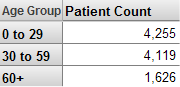
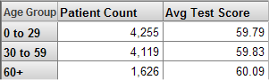
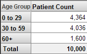
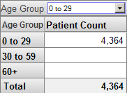
Most pivot tables simply display data for the members of one or more levels. For example, the Age Group level has the members 0 to 29, 30 to 59, and 60+. The following pivot table shows data for these members:
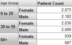
For another example, the following pivot table shows data for the Age Group and Gender levels (shown as the first and second columns respectively).
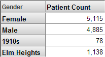
You can also drag and drop individual members for use as rows or columns. For example:
For more details on the options, see Using the Analyzer.
Member Names and Keys
Each member has both a name and an internal key. The compiler does not require either of these to be unique, even within the same level. Duplicate member names are legitimate in some cases, but you should check for and avoid duplicate member keys.
For an example of legitimate duplicate member names, consider that different people can have the same name, and you would not want to combine them into a single member. When a user drags and drops a member, the system uses the member key, rather than the name, in its generated query, so that the query always accesses the desired member.
Duplicate member keys, however, make it impossible to refer to each individual member. Given a member key, the system returns only the first member that has that key. You can and should ensure that your model does not result in duplicate member keys.
For information on the scenarios in which you might have duplicate member names and duplicate member keys, see Defining Member Keys and Names Appropriately.
Source Values
Each level is based on a source value, which is either a class property or an ObjectScript expression. For example, the Gender level is based on the Gender property of the patient. For another example, the Age Group level is based on an expression that converts the patient’s Age property to a string (0 to 29, 30 to 59, or 60+), depending on the age.
Hierarchies and Dimensions
In Business Intelligence, levels belong to hierarchies, which belong to dimensions. Hierarchies and dimensions provide additional features beyond those provided by levels.
Hierarchies are a natural and convenient way to organize data, particularly in space and time. For example, you can group cities into postal codes, and postal codes into countries.
There are three practical reasons to define hierarchies in Business Intelligence:
-
The system has optimizations that make use of them. For example, if you are displaying periods (year plus month) as rows or columns, and you then filter to a specific year, the query runs more quickly if your model defines years as the parent of periods.
-
You can use hierarchies within a pivot table as follows: If you double-click a member of a level, the system performs a drilldown to show the child members of that member, if any. For example, if you double-click a year, the system drills down to the periods within that year; for details, see Using the Analyzer.
-
MDX provides functions that enable you to work with hierarchies. For example, you can query for the child postal codes of a given country, or query for the other postal codes in the same country.
You can use these functions in handwritten queries; the Analyzer does not provide a way to create such queries via drag and drop.
A dimension contains one or more parent-child hierarchies that organize the records in a similar manner; for example, a single dimension might contain multiple hierarchies related to allergies. There is no formal relationship between two different hierarchies or between the levels of one hierarchy and the levels of another hierarchy. The practical purpose of a dimension is to define the default behavior of the levels that it contains — specifically the All level, which is discussed in the next subsection.
The All Level and the All Member
Each dimension can define a special, optional level, which appears in all the hierarchies of that dimension: the All level. If defined, this level contains one member, the All member, which corresponds to all records in the cube.
For example, the AgeD dimension includes one hierarchy with levels as follows:
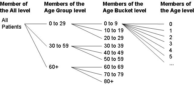
For a given dimension, you specify whether the All member exists, as well as its logical name and its display name. Within this dimension, the All member is named All Patients.
List-Based Levels
In Business Intelligence, unlike many other BI tools, you can base a level upon a list value. For example, a patient can have multiple diagnoses. The Diagnoses level groups patients by diagnosis. For example:
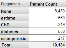
For a list-based level, any given source record can belong to multiple members. The pivot table shown here includes some patients multiple times.
See Also
Properties
Each level may define any number of properties. If a level has a property, then each member of that level has a value for that property; other levels do not have values for the property.
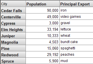
In the Patients sample, the City level includes the properties Population and Principal Export.
Each property is based on a source value, which is either a class property or an ObjectScript expression. For the City level, the properties Population and Principal Export are based directly on class properties.
You can use properties in queries in much the same way that you use measures. For example, in the Analyzer, you can use properties as columns (this example shows two properties):
In contrast to measures, properties cannot be aggregated. A property is null for all levels except for the level to which it belongs.
See Defining Properties.
Measures
A cube also defines measures, which show aggregate values in the data cells of a pivot table.
Each measure is based on a source value, which is either a class property or an ObjectScript expression. For example, the Avg Test Score measure is based on the patient’s TestScore property.
The definition of a measure also includes an aggregation function, which specifies how to aggregate values for this measure. Functions include SUM and AVG.
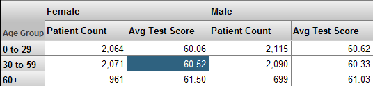
For example, the following pivot table shows the Patient Count measure and the Avg Test Score measure. The Patient Count measure counts the patients used in any context, and the Avg Test Score measure shows the average test score for the patients used in any context. This pivot table shows the value for these measures for the members of the Age Group level:
See Defining Measures.
Listings
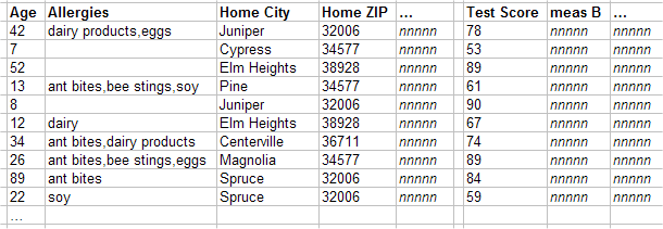
A cube can also contain listings. Each listing has a name and specifies the fields to display when the user requests that listing. The following shows an example:
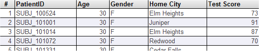
The records shown depend on the context from which the user requested the listing.
If you do not define any listings in a cube, then if a user requests a listing, the Analyzer displays the following message:
Error #5001: %ExecuteListing: this cube does not support drill through
See Defining Listings.
Also:
-
A cube can define individual listing fields with which users can create custom listings in the Analyzer. See Defining Listing Fields.
-
You can define listings outside of cube definitions (and without needing access to the Architect). See Defining Listing Groups.
Calculated Members
A calculated member is based on other members. You can define two kinds of calculated members:
-
A calculated measure is a measure is based on other measures. (In MDX, each measure is a member of the Measures dimension.)
For example, one measure might be defined as a second measure divided by a third measure.
The phrase calculated measure is not standard in MDX, but this documentation uses it for brevity.
-
A non-measure calculated member typically aggregates together other non-measure members. Like other non-measure members, this calculated member is a group of records in the fact table.
Calculated members are evaluated after the members on which they are based.
You can create calculated members of both kinds within the cube definition, and users can create additional calculated members of both kinds within the Analyzer.
Calculated Measures
It is very useful to define new measures based on other measures. For example, in the Patients sample, the Avg Allergy Count measure is defined as the Allergy Count measure divided by the Count measure. Consider the following pivot table:
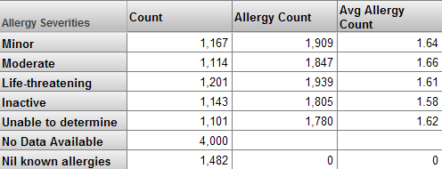
When this pivot table is run, the system determines the values for the Count and Allergy Count measures for each member of the Allergy Severities level; a later section of this page describes how the system does this. Then, for the Avg Allergy Count value for each member, the system divides the Allergy Count value by the Count value.
Non-Measure Calculated Members
For a non-measure calculated member, you use an MDX aggregation function to combine other non-measure members. The most useful function is %OR.
Remember that each non-measure member refers to a set of records. When you combine multiple members into a new member, you create a member that refers to all the records that its component members use.
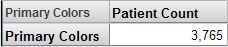
For a simple example, consider the ColorD dimension, which includes the members Red, Yellow, and Blue. These members access the patients whose favorite color is red, yellow, or blue, respectively. You can use %OR to create a single new member that accesses all three groups of patients.
For example:
See Also
Subject Areas
A subject area is a subcube with optional overrides to names of items. You define a subject area to enable users to focus on smaller sets of data without having to build multiple cubes. In a subject area, you can do the following:
-
Specify a filter that restricts the data available in the subject area. For information on filters, see the next section.
You can hardcode this filter, or you specify it programmatically, which means that you can specify it based on the $roles of the user, for example.
-
Hide elements defined in the cube so that the Analyzer displays a subset of them.
-
Define new names, captions, and descriptions for the visible elements.
-
Specify the default listing for the subject area.
-
Redefine or hide listings defined in the cube.
-
Define new listings.
You can then use the subject area in all the same places where you can use a cube. For example, you can use it in the Analyzer, and you can execute MDX queries on it in the shell or via the API.
Filters
In BI applications, it is critical to be able to filter data in pivot tables and in other locations. This section discusses the filter mechanisms in Business Intelligence and how you can use them in your application.
Filter Mechanisms
The system provides two simple ways to filter data: member-based filters and measure-based filters. You can combine these, and more complex filters are also possible, especially if you write MDX queries directly.
Member-Based Filters
A member is a set of records. In the simplest member-based filter, you use a member to filter the pivot table (for example, other contexts are possible, as this section describes later). This means that the pivot table accesses only the records that belong to that member.
For example, consider the following pivot table, as seen in the Analyzer:
Suppose that we apply a filter that uses the 0 to 29 member of the Age Group level. The resulting pivot table looks like this:
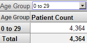
The Analyzer provides options to display null rows and columns. If we display null rows, the pivot table looks like this:
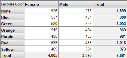
We can use the same filter in any pivot table. For example, consider the following unfiltered pivot table:
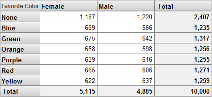
This pivot table shows the Patient Count measure although the headings do not indicate this. If we filter this pivot table in the same way as the previous one, we see this:
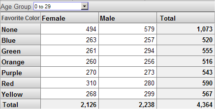
Notice that the total record count is the same in both cases; in both cases, we are accessing only patients that belong to the 0 to 29 member.
You can also use multiple members together in a filter, and you can combine filters that refer to members of different levels. Also, rather than choosing the members to include, you can choose the members to exclude.
Member-based filters are so easy to create and so powerful that it is worthwhile to create levels whose sole purpose is for use in filters.
Measure-Based Filters
The system supports searchable measures. With such a measure, you can apply a filter that considers the values at the level of the source record itself.
For the Patients sample, you can have a filter that accesses only the patients who have an encounter count of 10 or higher. If we use this filter in a pivot table, we might see this:
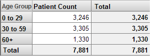
If we use the same filter in a different pivot table, we might see this:
In both cases, the total patient count is the same, because in both cases, the pivot table uses only the patients who have at least 10 encounters.
A searchable measure can also contain text values. With such measures, you can use the operators = <> and LIKE to filter the records.
More Complex Filters
It is possible to create more complex filters that combine member- and measure-based filters. The following shows an example of such a filter, as created in the Analyzer:
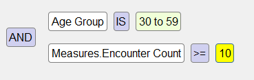
Internally, the query does not use AND and OR, but instead uses MDX syntax. All Business Intelligence filters use MDX syntax.
You can also create filters that use MDX functions. For example:
-
The FILTER function uses the aggregate values of a measure, rather than the lowest-level values which a measure-based filter uses. For example, you can use this to filter out patients who belong to cities that have fewer than 1000 patients.
In the Analyzer, the Levels option for a row or column uses this function internally.
-
The EXCEPT function can be used to remove specific members. The system uses this function when you create a member-based filter that excludes your selected members.
InterSystems MDX provides many other functions that perform set operations.
-
The TOPCOUNT and other functions access members based on their ranking.
For an introduction to MDX and a survey of your options, see Using InterSystems MDX. Also see InterSystems MDX Reference.
Using Filters
When you define a pivot table, you can specify how it is filtered. In practice, however, it is undesirable to create multiple similar pivot tables with different filters, because the pivot tables can become difficult to maintain. Instead, you can use any or all of the following tools:
-
In the Analyzer, you can define named filters, which you can then use in multiple pivot tables. A named filter is available in the Analyzer along with the contents of the cube or subject area (see the next item).
-
In the Architect, you can define subject areas that are filtered views of a base cube. Then when you create pivot tables, you start with a subject area rather than with the cube itself. These pivot tables are always filtered by the subject area filter, in addition to any filters that are specific to the pivot tables themselves.
In a subject area, you can specify a hardcoded filter, or you can customize a callback method to specify the filter at runtime (to base it on a value such as $roles, for example).
-
In the User Portal, when you create dashboards, you can include filter controls in them (this applies only to simple, member-based filters). Then the user can select the member or members to include or exclude.
Filters are always cumulative.
How the System Builds and Uses Fact Tables
When you compile a cube, the system generates a fact table and related tables. When you build a cube, the system populates these tables and generates their indexes. At runtime, the system uses these tables. This section describes this process. It includes the following topics:
The system does not generate tables for subject areas. A subject area uses the tables that have been generated for the cube on which the subject area is based.
Structure of a Fact Table
A fact table typically has one record for each record of the base table; this row is a fact. The fact contains one field for each level and one field for each measure. The following shows a sketch:
The field for a given level might contain no values, a single value, or multiple values. Each distinct value corresponds to a member of this level. The field for any given measure contains either null or a single value.
When the system builds this fact table, it also generates indexes for it.
The fact table does not contain information about hierarchies and dimensions. In the fact table, regardless of relationships among levels, each level is treated in the same way: the fact table contains one column for each level, and that column contains the value or values that apply to each source record.
By default, the fact table has the same number of rows as the base table. When you edit a cube class in an IDE, you can override its OnProcessFact() callback, which enables you to ignore selected rows of the base table. If you do so, the fact table has fewer rows than the base table.
Populating the Fact Table
When you perform a full build of a cube, the system iterates through the records of the base table. For each record, the system does the following:
-
Examines the definition of each level and obtains either no value, a single value, or multiple values.
In this step, the system determines how to categorize the record.
-
Examines the definition of each measure and obtains either no value or a single value.
The system then writes this data to the corresponding row in the fact table and updates the indexes appropriately.
When you perform a Selective Build, the system iterates through an existing fact table and updates or populates the selected columns.
When you build a cube upon which other related cubes depend, the system builds the related cubes as well, populating the related cubes’ fact tables in the appropriate order after it has done so for the independent cube.
Determining the Values for a Level
Each level is specified as either a source property or a source expression. Most source expressions return a single value for given record, but if the level is of type list, its value is a list of multiple values.
For a given record in the base table, the system evaluates that property or expression at build time, stores the corresponding value or values in the fact table, and updates the indexes appropriately.
For example, the Age Bucket level is defined as an expression that returns one of the following strings: 0-9, 10-19, 20-29, and so on. The value returned depends upon the patient’s age. The system writes the returned value to the fact table, within the field that corresponds to the Age Bucket level.
For another example, the Allergy level is a list of multiple allergies of the patient.
Determining the Value for a Measure
When the system builds the fact table, it also determines and stores values for measures. Each measure is specified as either a source property or an ObjectScript source expression.
For a given row in the base table, the system looks at the measure definition, evaluates it, and stores that value (if any) in the appropriate measure field.
For example, the Test Score measure is based on the TestScore property of the patients.
Determining the Value for a Property
When the system builds the fact table, it also determines values for properties, but it does not store these values in the fact table. In addition to the fact table, the system generates a table for each level (with some exceptions; see Details for the Fact and Dimension Tables). When the system builds the fact table, it stores values for properties in the appropriate dimension tables.
Using a Fact Table
Consider the following pivot table:
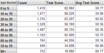
The first column displays the names of the members of the Age Bucket level. The first data column shows the Patient Count measure, the second data column shows the Test Score measure, and the last column shows the Avg Test Score measure. The Avg Test Score measure is a calculated member.
The system determines these values as follows:
-
The first row refers to the 0-9 member of the Age Bucket level. The system uses the indexes to find all the relevant patients (shown here with red highlighting) in the fact table:
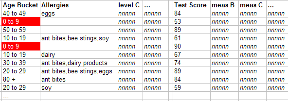
-
In the pivot table, the Patient Count column shows the count of patients used in a given context.
For the first cell in this column, the system counts the number of records in the fact table that it has found for the 0-9 member.
-
In the pivot table, the Test Score column shows the cumulative test score for the patients in a given context.
For the first cell in this column, the system first finds the values for the Test Score in the fact table that it has found for the 0-9 member:
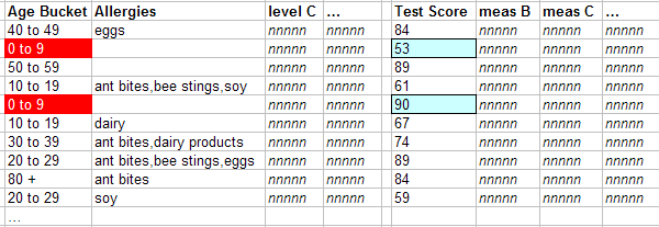
Then it aggregates those numbers together, in this case by adding them.
-
In the pivot table, the Avg Test Score column is meant to display the average test score for the patients in a given context.
The Avg Test Score measure is a calculated member, computed by dividing Test Score with Patient Count.
The system repeats these steps for all cells in the result set.
How the System Generates Listings
This section describes how the system uses the listings defined in the cube.
Within a pivot table, a user selects one or more cells.
The user then clicks the Listing button  , and the system displays a listing, which shows the values for the lowest-level records associated with the selected cells (also considering all filters that affect this cell):
To generate this display, the system:
-
Creates an temporary listing table that contains the set of source ID values that correspond to the facts used in the selected cells.
-
Generates an SQL query that uses this listing table along with the definition of your listing.
-
Executes this SQL query and displays the results.
Your cube can contain multiple listings (to show different fields for different purposes). When you create a pivot table in the Analyzer, you can specify which listing to use for that pivot table.
The listing query is executed at runtime and uses the source data rather than the fact table. Because of this, if the fact table is not completely current, it is possible for the listing to show a different set of records than you see in the fact table.