
Customizing Pivot Tables
This page describes how to further customize Business Intelligence pivot tables.
Also see Accessing the BI Samples.
Specifying Pivot Options
The Pivot Options dialog box provides many ways to customize the pivot table. To access this dialog box, click the Pivot Options button  . The Analyzer displays the following:
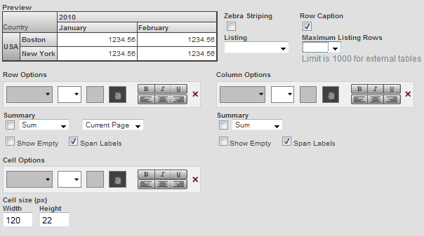
Here you can do the following:
-
Format the pivot table with zebra stripes. If you select Zebra Striping, the table is formatted with rows in alternating colors as follows:
-
Remove the captions for the rows. To do so, clear Row Caption.
-
Specify which listing to use for this pivot table. To do so, select a listing from the Listing drop-down menu.
-
Specify the maximum number of records to include in listings for this pivot table. To do so, specify a value for Maximum Listing Rows. The default is 1000.
-
Apply custom colors and font styles. To do so, use the drop-downs in Row Options, Column Options, or Cell Options. For example:
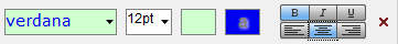
This style definition specifies that the font is in 12 pt, blue Verdana on a pale green background. The text is also bold and center-aligned.
If you specify a custom color for the cell background in Cell Options, the system ignores the Zebra Striping option.
-
Use the Span Labels options to control whether labels are spanned.
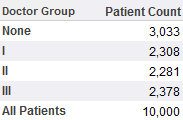
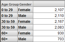
When you display the table in a nested format, the labels are spanned by default. For example:
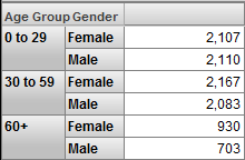
You can instead repeat the relevant labels, as follows:
-
Use the Show Empty options to control whether empty rows and columns are displayed.
-
Control the size of the data cells. To do so, type the width in pixels into Width and the height in pixels into Height.
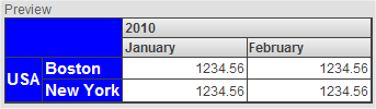
As you make changes, the Preview area is updated to demonstrate the changes. For example:
If you have enabled the %SQLRESTRICT dimension for a cube, you will see the SQL Restriction field. If you wish to apply an SQL Restriction for the current pivot table, enter a valid SQL SELECT statement or WHERE clause. For more information, see %FILTER Clause.
Customizing Pivot Table Items
The Analyzer displays an Advanced Options button  in the Rows, Columns, and Measures boxes, next to each item in those boxes. The same button is also available for the Rows and Columns boxes.
For example:
If you click any of these buttons, you see the following dialog box—depicted here with only its top part—or a variation of it (the details are different for measures).
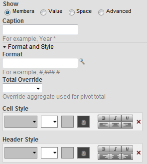
The following sections describe changes you can make.
You can specify formatting in multiple places. If you specify different formatting, the following rules control which formatting options are used:
-
Wherever possible, all the formatting is used. For example, if you specify the typeface to use for rows and the color to use for columns, both format options are applied.
-
Formatting specified for a measure in a pivot table takes precedence over formatting specified elsewhere.
-
Formatting specified for columns takes precedence over formatting specified for rows or the entire pivot table.
-
Formatting specified for rows takes precedence over formatting specified for the entire pivot table.
-
Formatting specified in the pivot table takes precedence over formatting specified in a measure definition (other model elements do not have format options).
Displaying a Constant Row or Column
You can display a constant value rather than the selected item. To do so:
-
Click the Advanced Options button
next to the item. -
Click Value.
-
Type a value into Value. For example:
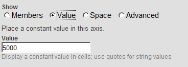
-
Click OK.
You might also want to specify a different caption; see Specifying New Captions, later in this page.
Specifying a Spacer Row or Column
You can display a spacer row or column rather than the selected item or items. To do so:
-
Click the Advanced Options button
next to the item. -
Click Space.
-
Click OK.
The following shows an example:
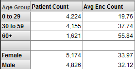
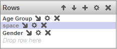
For this pivot table, the Rows definition is as follows:
Displaying an Different Set for Rows or Columns
You can display an alternative set of elements rather than the selected item or items. To do so:
-
Click the Advanced Options button
next to the item. -
Click Advanced.
-
Type an MDX set expression into MDX Expression.
For information, see Using InterSystems MDX.
-
Click OK.
Specifying New Captions
To specify new captions:
-
Click the Advanced Options button
next to the item or in the header of the Rows or Columns box, as appropriate. -
Type a value into Caption.
To include the original name in the caption, use an asterisk (*) at the appropriate position.
-
Click OK.
For example:
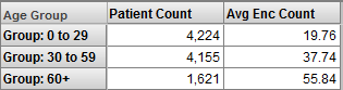
In this case, Caption is Group: *
Specifying a Format String
A format string controls how numbers are displayed and can also specify colors to use. To specify the format string for an item:
-
Click the Advanced Options button
next to the item or in the header of the Rows or Columns box, as appropriate. -
Click the Find button
 next to Format.
The system displays a dialog box that includes the following fields:

Here:
-
Positive piece specifies the format to use for positive values.
-
Negative piece specifies the format to use for negative values.
-
Zero piece specifies the format to use for zero.
-
Missing piece specifies the format to use for missing values.
In each of these, Format string specifies the numeric format, and Color specifies the color.
-
-
Specify values as needed (see the details after these steps).
-
Click OK.
Format String Field
The Format string field is a string that includes one of the following base units:
| Base Unit | Meaning | Example |
|---|---|---|
| # | Display the value without the thousands separator. Do not include any decimal places. | 12345 |
| #,# | Display the value with the thousands separator. Do not include any decimal places. This is the default display format for positive numbers. | 12,345 |
| #.## | Display the value without the thousands separator. Include two decimal places (or one decimal place for each pound sign after the period). Specify as many pound signs after the period as you need. | 12345.67 |
| #,#.## | Display the value with the thousands separator. Include two decimal places (or one decimal place for each pound sign after the period). Specify as many pound signs after the period as you need. | 12,345.67 |
You can include additional characters before or after the base unit.
-
If you include a percent sign (%), the system displays the value as a percentage. That is, it multiplies the value by 100 and it displays the percent sign (%) in the position you specify.
-
Any other characters are displayed as given, in the position you specify.
The following table shows some examples:
| Example formatString | Logical Value | Display Value |
|---|---|---|
| formatString="#,#;(#,#);"
Note that this corresponds to the default way in which numbers are displayed. |
6608.9431 | 6,609 |
| –1,234 | (1,234) | |
| formatString="#,#.###;" | 6608.9431 | 6,608.943 |
| formatString="#%;" | 6 | 600% |
| formatString="$#,#;($#,#);" | 2195765 | $2,195,765 |
| –3407228 | ($3,407,228) |
Color Piece
For the Color field, specify either of the following:
-
A CSS color name such as MediumBlue or SeaGreen. You can find these at https://www.w3.org/TR/css3-color/Opens in a new tab and other locations on the Internet.
-
A hex color codeOpens in a new tab such as #FF0000 (which is red).
-
An RGB value such as rgb(255,0,0) (which is red).
Specifying Cell and Header Styles
To specify the cell and header styles for an item:
-
Click the Advanced Options button
next to the item or in the header of the Rows or Columns box, as appropriate. -
Select values in the Cell Style and Header Style groups. These enable you to specify the style of the cells and the headers, respectively:

To use these options, click each drop-down and select a value. For example:
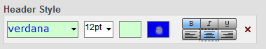
This style definition specifies that the header is in 12 pt, blue Verdana on a pale green background. The header is also bold and center-aligned.
-
Click OK.
Sorting and Filtering Members
You can filter and sort the members of a level or named set in various ways. To do so:
-
Click the Advanced Options button
next to a level or named set or in the header of the Rows or Columns box, as appropriate. -
Specify the following options as needed:
-
Filter members — Select this to filter the members by a measure value. Then select a measure and a comparison operator and type a value.
-
Sort members — Select this to sort the members. Then select the measure by which to sort them. Click Ascending or Descending to control how the members are sorted.
-
Return the first n members — Select this to select a subset from the beginning of the set. Then type an integer into Count.
When you use this option, the system first uses any settings you specified for the Filter members and Sort members options.
-
-
Click OK.
Specifying Alternative Aggregation Methods for a Measure
For any cell in a pivot table, each measure is aggregated from the lowest-level data. Aggregation methods include sum, average, maximum value, and others. By default, the system uses the aggregation method specified in the measure definition. You can specify an alternative method.
Similarly, if you add a summary row or column, you specify how to aggregate the displayed values into a single number for that summary row or column. You can specify an alternative method for this as well.
To specify alternative aggregation methods for a measure:
-
Click the Advanced Options button
next to the measure. -
Specify either or both of the following options:
-
Measure Aggregate specifies how this measure is aggregated from a set of values in your data.
The choices are SUM, AVG, MIN, MAX, and COUNT.
-
Total Override specifies how the displayed measure values are aggregated for any summary rows or columns.
The choices are Sum, Count, Min, Max, Average, % of Total, and None.
-
-
Click OK.
See also Adding a Summary Row or Column.
Customizing Double-Click Drilldown
By default, when you double-click a row in a pivot table, the system drills down to the next lowest level in the hierarchy, if any (see Drilldown via Double-Click). You can customize this behavior. To do so:
-
Click the Advanced Options button
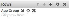
in the header of the Rows box. -
Expand the Drilldown Options group if that is collapsed.
-
For Drilldown Expression, specify one or more MDX set expressions, one per line. For example:
colord.h1.[favorite color].members
gend.h1.gender.members
To specify MDX set expressions, you can do either of the following:
-
Type the expression directly into Drilldown Expression. Use a line return to establish required line breaks between items.
-
Use the Expression Builder. To access this tool, click the plus sign
 next to Drilldown Expression. The left area lists the contents of the cube, including all measures and levels. The right area displays the expression that you are creating. To add an item to the expression, drag and drop it from the left area to the expression. The item is added to the end of the expression, and you might need to move it to a different part of the expression.
Click the plus sign each time you add an item to the expression. Using the plus sign (rather than a line return) causes the Expression Builder to establish and preserve the required line breaks between items.
Typically you use set expressions of the form [dimension].[hierarchy].[level].MEMBERS, where dimension is the logical name of a dimension, hierarchy is the logical name of a hierarchy, and level is the logical name of a level. This expression represents the members of the given level.
If these identifiers do not include spaces, you can omit the square brackets. Also, the expression is not case-sensitive.
The first set expression controls what happens when the user double-clicks the first time. Specifically, when the user double-clicks the first time, the system creates a new query that uses this set expression for rows and that is filtered to the given context.
Similarly, the second expression controls what happens when the user double-clicks the second time, and so on.
The Drilldown Expression option overrides any other drilldown behavior in this pivot table. That is, if a level is in a hierarchy, the hierarchy drilldown behavior does not occur for this pivot table.
-
-
Click OK.
Disable drilldown: If you wish at any time to disable (but preserve) this drilldown expression, select the Disable drilldown check box. Click OK. This prevents use of the drilldown expression when you double-click a row in this pivot table. It also prevents modification of the drilldown expression. To re-activate the drilldown expression, clear the Disable drilldown check box.
For a Drilldown Expression example, see Custom Double-Click Drilldown.
The same option is available in the Advanced Options button in the header of the Columns box. This option is ignored by default but is used if you pivot the table (via the Transpose button  ) and then perform double-click drilldown.
Applying Conditional Formatting
You can apply conditional formatting, which can add color, text, or graphics to pivot table cells. To do so, you create rules that examine the values in the cells. This conditional formatting overrides any customization you added to the pivot table.
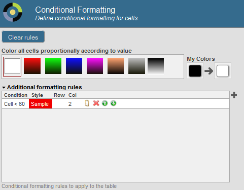
To do so, click the Conditional Formatting button  in the toolbar. The system displays a dialog box like the following (in this example, one rule has been specified):
Here, you can do the following:
-
Clear all conditional formatting. To do so, click Clear rules.
-
Apply an overall color, based on values in the cells. To do so, click a button in the section Color all cells proportionally according to value. See Applying an Overall Color.
-
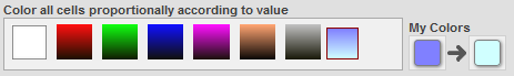
Define a custom gradient for use with the option Color all cells proportionally according to value. To define a custom gradient, use the two buttons displayed below My Colors. Click the first one and select a color to use at the bottom of the range. Click the second one and select a color to use at the top of the range. When you are done, the dialog box displays your gradient next to the predefined gradients. For example:
-
Create formatting rules. See Adding a Rule.
-
Change the order of the rules. To do so, click the up or down arrows in the row for a rule.
-
Delete a rule. To do so, click the X button in the row for that rule.
-
Reconfigure a rule. To do so, click the Reconfigure button
 in the row for that rule.
 -
Apply the existing rules while leaving this dialog box open. To do so, click Apply.
-
Apply the existing rules and exit this dialog box. To do so, click OK.
-
Close this dialog box without making changes. To do so, click Cancel.
Rules are applied in the same order that they are listed here. If a later rule contains formatting information that is inconsistent with an earlier rule, the system uses the formatting specified in the later rule.
Applying an Overall Color
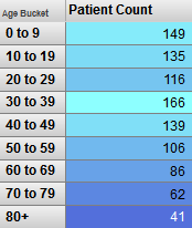
If you click a button in the section Color all cells proportionally according to value, the cells are colored according to their values. This works as follows: Each button displays a gradient of colors. To assign a color to a cell, the system examines the range of values of the cells. If a value is at the bottom of this range, the system uses the color that is shown at the top of the gradient button (a dark blue in the following example). If a value is at the top of this range, the system uses the color that is shown at the bottom of the gradient button (a light blue in the following example). For other values, the system uses an intermediate color. The following shows an example:
Adding a Rule
To add a rule, click the plus sign button. The system displays a dialog box where you can specify the rule details (in this example, one rule has been specified):
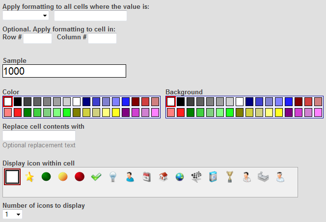
Here you can do the following:
-
Specify the numeric comparison for the rule to use. A rule compares the value in each cell (or in specific cells) to a constant, using an operator. For example:
cell_value > 50For each cell where this rule is true, the rule is applied. All the display details of the rule are applied to that cell.
To specify the numeric comparison, do the following:
-
Select an operator from the first drop-down menu.
-
Type a numeric constant into the field to the right of that.
-
-
Optionally specify which row, which column, or both the rule applies to. To do so, type a number into Row #, Col #, or both.
-
Optionally specify the text color to use when the rule is true. To do so, click a button in the Color section. If you select the left-most button, the system uses the default color.
-
Optionally specify the background color to use when the rule is true. To do so, click a button in the Background Color section. If you select the left-most button, the system uses the default color.
-
Optionally specify replacement text to display when the rule is true, instead of the actual cell value. To do so, type text into Replace cell contents with.
-
Optionally specify an icon to display when the rule is true, instead of the actual cell value. To do so, click a button in Display icon in cell. This area lists the system icons, followed by any custom icons defined by the implementers. (For information on adding icons that can be used here, see Creating Icons.)
If you select the left-most button, the system does not display an icon.
To display multiple icons, click a number from the Number of icons to display list.
The bottom of the dialog box shows a preview of the formatting.
Specifying the Print Settings
To specify the print options for a given pivot table:
-
Display that pivot table in the Analyzer.
-
Click the Print Options button
 .
. -
Click Page Setup.
-
Specify options as described in Customizing Print Settings for a Widget.
-
Click OK.
-
Save the pivot table.
For comments on printing, see Printing Pivot Tables.
Note that when you create dashboards, you can specify print settings in the dashboards as well. See Customizing Print Settings for a Widget.
Specifying the MDX Query Manually
Sometimes it is useful to see and then modify the MDX query that the system generates for a pivot table. To do so:
-
Click the Query Text button
 .
.The system then displays a dialog box that displays the query used by this pivot table.
-
If you want to use a different query, click Manual Mode.
-
Edit the query. See the following subsection for an example.
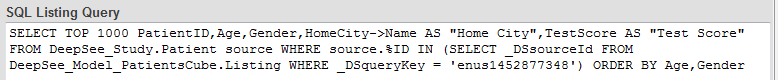
If you had displayed a detail listing, the bottom area of this dialog box also displays the listing query that the system used:
-
Click OK.
When the Analyzer displays a pivot table that is defined by a manually edited or manually entered MDX query, the Query Text button changes to the following:  . Also, the Rows, Columns, and Measures boxes are grayed out. You cannot use locally defined calculated members unless you also add the appropriate WITH clause to your query. You can, however, drag items to the Filters box; the system applies these filters but does not modify the manual query text. That is, the base query and its filters are stored separately within the pivot table definition.
You can also use the Query Text option to copy and paste the query (for example, to use in the MDX shell).
Modifying Details of the 80/20 Suppression Option
For example, if you had used the 80/20 suppression option, the MDX query might look like this (with harmless line breaks added):
SELECT
NON EMPTY {[Measures].[Amount Sold],[Measures].[Units Sold],[Measures].[%COUNT]}
ON 0,
NON EMPTY
{TOPPERCENT([Product].[P1].[Product Name].Members,80),
%LABEL(SUM(BOTTOMPERCENT([Product].[P1].[Product Name].Members,20)),"Other",,,,"font-style:italic;")}
ON 1
FROM [HoleFoods]
For the TOPPERCENT and BOTTOMPERCENT functions:
-
The first argument specifies the set of members to use.
-
The second argument specifies the percentage.
-
The third argument (omitted in the preceding example) specifies the measure to use for ranking the members.
To change the percentages, change the second arguments for TOPPERCENT and BOTTOMPERCENT. For example:
SELECT
NON EMPTY {[Measures].[Amount Sold],[Measures].[Units Sold],[Measures].[%COUNT]} ON 0,
NON EMPTY
{TOPPERCENT([Product].[P1].[Product Name].Members,90),
%LABEL(SUM(BOTTOMPERCENT([Product].[P1].[Product Name].Members,10)),"Other",,,,"font-style:italic;")}
ON 1
FROM [HoleFoods]
For details on MDX, see Using InterSystems MDX and InterSystems MDX Reference.