
Principles and Recommendations
This page discusses core principles and other recommendations for your InterSystems IRIS® data platform Business Intelligence models.
Also see Accessing the Business Intelligence Samples.
Choosing a Base Table
When defining a cube, the first step is to choose the class to use as the base class for that cube. The key point to remember is this: Within the cube, any record count refers to a count of records in this class (as opposed to some other class referenced within the cube). Similarly, the selection of the base class determines the meaning of all measures in the cube.
For example:
-
If the base class is Transactions, transactions are counted. In this cube, you can have measures like the following:
-
Average broker fee per transaction (or average for any group of transactions)
-
Average transaction value per transaction (or average for any group of transactions)
-
-
If the base class is Customers, customers are counted. In this cube, you can have measures like the following:
-
Average broker fee per customer (or average for any group of customer)
-
Average transaction value per customer (or average for any group of customers)
-
You can have multiple cubes, each using a different base class, and you can use them together in dashboards.
Choosing the Form of the Base Table
It is also important to consider the form of the base table. The following table summarizes the key considerations:
| Base Table | Support for DSTIME? | Support for Listings? |
|---|---|---|
| Local persistent class (other than a linked table) | Yes | Yes |
| Linked table | No | Yes |
| Data connector that uses local tables | No | Yes |
| Data connector that uses linked tables | No | No |
The DSTIME feature is the easiest way to keep the corresponding cube current. When this feature is not available, other techniques are possible. For details, see Keeping the Cubes Current.
Avoiding Large Numbers of Levels and Measures
InterSystems IRIS® data platform imposes a maximum limit on the number of levels and measures on a cube, because there is a limit on the number of indexes in a class. For information on this limit (which may increase over time), see General System Limits. For information on the number of indexes that the system creates for levels and measures, see Details for the Fact and Dimension Tables.
It is also best to keep the number of levels and measures much smaller than required by this limit, because an overly complex model can be hard to understand and use.
Defining Measures Appropriately
The value on which a measure is based must have a one-to-one relationship with the records in the base table. Otherwise, the system would not aggregate that measure suitably. This section demonstrates this principle.
Measures from Parent Tables
Do not base a measure on a field in a parent table. For example, consider the following two tables:
-
Order — Each row represents an order submitted by a customer. The field SaleTotal represents the total monetary value of the order.
-
OrderItem — Each row represents an item in that order. In this table, the field OrderItemSubtotal represents the monetary value of this part of the order.
Suppose that we use OrderItem as the base table. Also suppose that we define the measure Sale Total, based on the parent’s SaleTotal field. The goal for this measure is to display the total sale amount for all the sales of the selected order items.
Let us consider the contents of the fact table. The following shows an example:
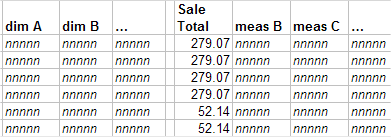
The first four rows represent the items in the same order. The next two rows represent the items of another order, and so on.
Suppose that this model has a dimension called Item Type. Let us examine what happens when the system retrieves records for all items of type R:
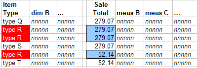
To compute the value of the Sale Total measure for type R, the system adds together the three values shown here: 279.07, 279.07, and 52.14. But this action double-counts one of the orders.
Depending on the case, the Sale Total measure might aggregate correctly; that is, it might show the correct total sales figure for the selected order items. But you cannot ensure that the measure does this, because you cannot prevent double-counting as shown as in this example.
Measures from Child Tables
You can use a value in a child table as the basis of a measure, but to do so, you must aggregate that value across the relevant rows of the child table.
Consider the following two tables:
-
Customer — Each row represents a customer.
-
Order — Each row represents a customer order. The field SaleTotal represents the total monetary value of the order.
Suppose that we use Customer as the base table, and that we want to create a measure based on the SaleTotal field.
Because a customer potentially has multiple orders, there are multiple values for SaleTotal for a given customer. To use this field as a measure, we must aggregate those values together. The most likely options are to add the values or to average them, depending on the purpose of this measure.
Understanding Time Levels
A time level groups records by time; that is, any given member consists of the records associated with a specific date and time. For example, a level called Transaction Date would group transactions by the date on which they occurred. There are two general kinds of time levels, and it is important to understand their differences:
-
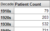
Timeline-based levels. This kind of time level divides the timeline into adjacent blocks of time. Any given member of this level consists of a single block of time. Or, more accurately, the member consists of the records associated with that block of time. For a level called Transaction Quarter Year, the member Q1-2011 would group all the transactions that occurred in any of the dates that belong to the first quarter of 2011.
This kind of level can have any number of members, depending on the source data.
-
Date-part based levels. This kind of time level considers only part of the date value and ignores the timeline. Any given member consists of multiple blocks of time from different parts of the timeline, as shown in the following figure. Or, more accurately, the member consists of the records associated with those blocks of time. For a level called Transaction Quarter, the member Q1 would group all the transactions that occurred in any of the dates that belong to the first quarter of any year.
This kind of level has a fixed number of members.
The following figure compares these kinds of time levels:

You can use these kinds of levels together without concern; the engine will always return the correct set of records for any combination of members. However, there are two typical sources of confusion:
-
If you define hierarchies of time levels (that is, hierarchies that contain more than one level), you must think carefully about what you include. As noted in the next section, MDX hierarchies are parent-child hierarchies. Any member in the parent level must contain all the records of its child members.
This means, for example, that you can use the Transaction Year level as the parent of the Transaction Quarter Year level, but not of the Transaction Quarter level. To see this, refer to the preceding figure. The Q1 member refers to the first quarters of all years, so no single year can be the parent of Q1.
Time Levels and Hierarchies gives guidelines on appropriate time hierarchies.
-
Some MDX functions are useful for levels that represent the timeline, but are not useful for levels that represent only a date part. These functions include PREVMEMBER, NEXTMEMBER, and so on. For example, if you use PREVMEMBER with Q1–2011, the engine returns Q4–2010 (if your data contains the applicable dates). If you use PREVMEMBER with Q1, there is nothing useful to return.
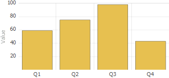
You might want to try defining the following flexible approach: Define a Year level so that you have one level that represents the timeline. Define all other time levels as date-part levels. Then you can use these levels together as in the following example:
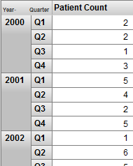
This pivot table uses a combination of Year (a timeline level) and Quarter (a date-part level) for rows. The Quarter level is also useful on its own, because it can provide information on quarter-by-quarter patterns. The sample data in SAMPLES does not demonstrate this, but there are many kinds of seasonal activity that you could see this way. The following shows an example:
Defining Hierarchies Appropriately
In any hierarchy, pay attention to the order of the levels as shown in the Architect. A level is automatically a child of the previously listed level in that hierarchy. For example, consider the HomeD dimension from the Patients sample:
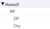
The ZIP level is the parent of the City level. More precisely, each member of the ZIP level is the parent of one or more members of the City level. (In reality, there is a many-to-many relationship between ZIP codes and cities, but the Patients sample is simplistic, and in this sample, ZIP codes represent larger areas than cities.)
In your hierarchies, the first level should be the least granular, and the last one should be the most granular.
MDX hierarchies are parent-child hierarchies. To enforce this rule, the system uses the following logic when it builds the cube:
-
For the first level defined in a hierarchy, the system creates a separate member for each unique source value.
-
For the levels after that, the system considers the source value for the level in combination with the parent member.
For example, suppose that the first level is State, and the second level is City. When it creates members of the City level, the system considers both the city name and the state to which that city belongs.
The internal logic is slightly different for time hierarchies, but the intent is the same.
What Happens if a Hierarchy Is Inverted
In contrast, suppose that we move the City level so that it is before the ZIP level in the cube, recompile, and rebuild. If we use the ZIP level for rows in a pivot table, we see something like the following:
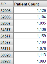
In this case, the system has created more than one member with the same name, because it assumes that (for example) there are two ZIP 32006 codes, which belong to different cities.
In this case, it is obviously incorrect to have multiple members with the same name. In other scenarios, however, it is legitimate to have multiple members with the same name. For example, different countries can have cities with the same name. That is, if you have duplicate member names, that can indicate an inverted hierarchy, but not in all cases.
Time Hierarchies
MDX hierarchies are parent-child hierarchies. All the records for a given child member must be contained in the parent member as well. It is important to carefully consider how to place time levels into hierarchies. See the previous section. Also Time Levels and Hierarchies, gives guidelines on appropriate time hierarchies.
Defining Member Keys and Names Appropriately
Each member has both a name and an internal key. By default, these are the same, except for time levels. Both of these identifiers are strings. When you define your model, you should consider the following items:
-
Very long member keys can trigger a SUBSCRIPT error. If you are working with source data that yields very long member keys, you may implement source processing in your level's sourceExpression to ensure the data is preserved in a manner of your choosing.
-
It can be correct to have duplicate member names. Different people, for example, can have the same name. When a user drags and drops a member, the system uses the member key, rather than the name, in its generated query.
-
InterSystems recommends that you ensure that member keys are unique in each level. Duplicate member keys make it difficult to refer to all the individual members.
In particular, if you have duplicate member keys, users cannot reliably drill down by double-clicking.
-
To help users distinguish the members, if a level has multiple members with the same name, InterSystems also recommends that you add a property to the level whose value is the same as the key. To do so, simply base the property on the same source property or source expression that the level uses.
Then the users can display the property to help distinguish the members.
Or add a tooltip to the level, and have that tooltip contain the member key.
The following sections describe the scenarios in which you might have duplicate member keys and names.
Ways to Generate Duplicate Member Keys
Duplicate member keys are undesirable. If you have duplicate member keys, users cannot reliably drill down by double-clicking.
Except for time levels, each unique source value for a level becomes a member key. (For time levels, the system uses slightly different logic to generate unique keys for all members.)
If there is a higher level in the same hierarchy, it is possible for the system to generate multiple members with the same key. See Ensuring Uniqueness of Member Keys.
Ways to Generate Duplicate Member Names
Duplicate member names may or may not be undesirable, depending on your business needs.
Except for time levels, each unique source value for a level becomes a member name, by default. (For time levels, the system generates unique names for all members.)
There are only two ways in which the system can generate multiple members with the same name:
-
There is a higher level in the same hierarchy. This higher level might or might not be suitable. See Defining Hierarchies Appropriately.
-
You have defined a level as follows:
-
The member names are defined separately from the level definition itself.
-
The member names are based on something that is not unique.
-
Note that InterSystems IRIS does not automatically trim leading spaces from string values as it builds the fact table. If the source data contains leading spaces, you should use a source expression that removes those. For example:
$ZSTRIP(%source.myproperty,"<W")
Otherwise, you will create multiple members with names that appear to be the same (because some of the names have extra spaces at the start).
Avoiding Very Granular Levels
For users new to Business Intelligence, it is common to define a level that has a one-to-one relationship with the base table. Such a level is valid but is not particularly useful, unless it is also combined with filters to restrict the number of members that are seen.
A very granular level has a huge number of members (possibly hundreds of thousands or millions), and Business Intelligence is not designed for this scenario.
For example, suppose that we modified the Patient sample to have a Patient level. Then we could have a pivot table like this:
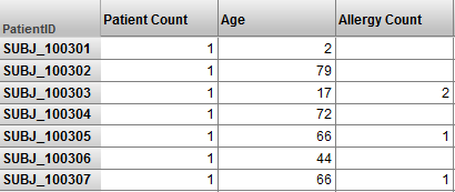
This is valid but an SQL query would produce the same results more efficiently. Consider the processing that is described in How Business Intelligence Builds and Uses Fact Tables. (That description gives the conceptual flow rather than the actual processing, but the overall idea is the same.) That processing is intended to aggregate values together as quickly as possible. The pivot table shown above has no aggregation.
If you need a pivot table like the one shown here, create it as an SQL-based KPI. See Advanced Modeling for InterSystems Business Intelligence.
Using List-Based Levels Carefully
In Business Intelligence, unlike many other BI tools, you can base a level upon a list value. Such levels are useful, but it is important to understand their behavior.
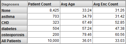
For example, a patient can have multiple allergies. Each allergy has an allergen and a severity. Suppose that the base table is Patients and the model includes the Allergies and Allergy Severity levels. We could create a pivot table that looks like this:
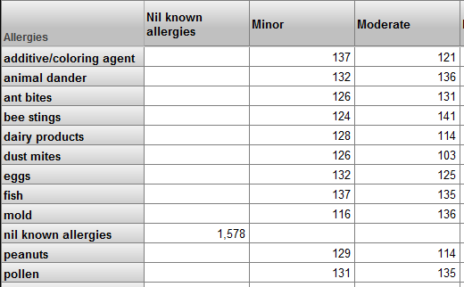
Upon first seeing this pivot table, the user might think that this pivot table shows correlations between different sets of patient allergies. It does not.
This pivot table, as with all other pivot tables in this cube, shows sets of patients. For example, the ant bites row represents patients who have an allergy to ant bites. The Minor column represents patients who have at least one allergy that is marked as minor. There are 126 patients who have an allergy to ant bites and who have at least one allergy that is marked as minor. This does not mean that there are 126 patients with minor allergies to ant bites.
It is possible to create a pivot table that does show correlations between different sets of patient allergies. To do so, however, you would have to define a model based on the patient allergy, rather than the patient.
When you use a list-based level in a filter, the results require careful thought. Consider the following pivot table:
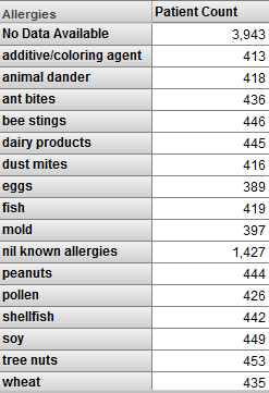
This pivot table shows patients, grouped by allergy. Now suppose that we apply a filter to this pivot table, and the filter selects the fish member:
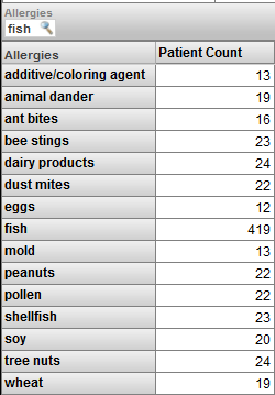
Now we are viewing only patients who have an allergy to fish. Note the following:
-
The pivot table shows the fish member. For this member, the patient count is the same as in the previous pivot table.
-
It also shows some other members of the Allergies level. For these members, the patient count is lower than in the previous pivot table.
-
The pivot table does not include the No Data Available member of the Diagnoses level. Nor does it include the Nil Known Allergies member.
To understand these results, remember that we are viewing only patients who are allergic to fish, and this is not the same as viewing only the fish allergy. The patients who are allergic to fish are also allergic to other things. For example, 13 of the patients who are allergic to fish are also allergic to additives/coloring agents.
If we change the filter to select only the No Data Available member, we see this:
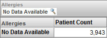
In this case, we are viewing only the patients who do not have any recorded allergy. By definition (because of how this level is defined), there is no overlap of these patients with the patients who have specific allergies.
List-based levels cannot have child or parent levels.
Handling Null Values Correctly
For any measure or level, the source value could potentially be null in some cases. It is important to understand how the system handles nulls and to adjust your model according to your business needs and usability requirements.
Null Values in a Measure
For a measure, if the source value is missing for a given record, the system does not write any value into the measure column of the fact table. Also, the system ignores that record when aggregating measure values. In most scenarios, this is appropriate behavior. If it is not, you should use a source expression that detects null values and replaces them with a suitable value such as 0.
Null Values in a Level
For a level, if the source value is missing for a given record in the base class, the system automatically creates a member to contain the null values (with one exception). You specify the null replacement string to use as the member name; otherwise, the member is named Null.
The exception is computed dimensions, which are discussed in Advanced Modeling for InterSystems Business Intelligence. The replacement string has no effect in this case.
Usability Considerations
It is also useful to consider how users see and use the model elements. This section explains how the Analyzer and pivot tables represent model elements and concludes with some suggestions for your models.
Consider How Dimensions, Hierarchies, and Levels Are Presented
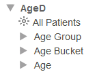
The Model Contents area of the Analyzer displays each dimension and the levels in it, but does not display the hierarchies (for reasons of space). For example:
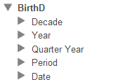
Therefore, a user working in the Analyzer does not necessarily know which levels are related via hierarchies.
If a level is used for rows, then the name of the level appears as the column title. For example:
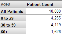
If a dimension is used for rows, the name of the dimension appears as the column title. Also, the system uses an MDX function that gets the All member for the dimension, as well as all members of the first level defined in that dimension:
Consider How to Use All Members
The Model Contents area displays every All member. For example:
In the Analyzer, users can drag and drop the All member, in the same way they can drag any other member.
The All member for one dimension is equivalent (except for its name) to the All member for any other dimension. If it has a suitably generic name, an All member is useful as the bottom line. For example:
Considerations with Multiple Cubes
If you find that you need to define multiple cubes to analyze one area of your business, consider the following points:
-
If you have a large number of cubes, relationships are often quite useful. Rather than defining the same dimension repeatedly in different cubes (with different definitions), you can define it in a single place. This is more convenient for development and lessens the amount of disk space that is needed.
The slight disadvantage of relationships is that when you rebuild an independent cube, all of the cubes which depend upon it must also be rebuilt, in the appropriate order. Fortunately, Business Intelligence rebuilds a cube’s dependents automatically.
-
If you need pivot tables that display measures from multiple cubes, you must define shared dimensions and a compound cube. A compound cube is the only way to use measures together that belong to different cubes.
Recommendations
The following recommendations may also be useful to you, depending on your business needs:
-
Decide whether you will use dimensions directly in pivot tables. If so, assign user-friendly names to them (at least for display names).
If not, keep their names short and omit spaces, to enable you to write MDX queries and expressions more easily.
Also, use a different name for the dimension than for any level in the dimension, in order to keep the syntax clear, if you need to view or create MDX queries or expressions.
-
Hierarchy names are not visible in the Analyzer or in pivot tables. If you use short names (such as H1), your MDX queries and expressions are shorter and easier to read.
-
Define only one hierarchy in any dimension; this convention gives the users an easy way to know if the levels in a dimension are associated with each other.
-
Define an All member in only one dimension. Give this All member a suitably generic name, such as All Patients. Depending on how you intend to use the All member, another suitable name for it might be Total or Aggregate Value.
-
Use user-friendly names for levels, which are visible in pivot tables.
-
You can have multiple levels with the same name in different hierarchies. Pivot tables and filters, however, show only the level name, so it is best to use unique level names.
-
Specify a value for the Field name in fact table option for each applicable level and measure; this option does not apply to time levels, NLP levels, or NLP measures. Take care to use unique names.
It is much easier to troubleshoot when you can identify the field in which a given level or measure is stored, within the fact table.
For information, see Details for the Fact and Dimension Tables.